自然策略梯度（NPG）¶

论文链接： https://proceedings.neurips.cc/paper_files/paper/2001/file/4b86abe48d358ecf194c56c69108433e-Paper.pdf

自然策略梯度（Natural Policy Gradient，NPG）是一种深度强化学习算法，其目标是利用 Fisher 信息矩阵（Fisher Information Matrix，FIM）优化策略，并直接最大化期望回报。该算法由 Sham Kakade 于 2001 年提出。 NPG 已被广泛应用于机器人、金融和博弈论等多种强化学习问题。

下表列出了 NPG 算法的一些基本特征：

NPG 的特征	是否具备	说明
同策略（On-policy）	✅	评估策略与目标策略相同。
异策略（Off-policy）	❌	评估策略与目标策略不同。
无模型（Model-free）	✅	无须预先构建环境动力学模型。
基于模型（Model-based）	❌	需要使用环境模型训练策略。
离散动作	✅	可处理离散动作空间。
连续动作	✅	可处理连续动作空间。

策略优化¶

NPG 的核心思想是计算期望回报关于策略参数的梯度，以优化策略。将策略记为 \(\pi(\theta)\)，其中 \(\theta\) 为参数向量，则期望回报 \(J(\theta)\) 表示为：

\[ J(\theta) = \mathbb{E}_{\pi(\theta)}[R] = \sum_s \rho^\pi(s) \sum_a \pi(a; s, \theta) R(s, a) \]

其中，\(\rho^\pi(s)\) 是策略 \(\pi\) 对应的平稳分布。期望回报关于 \(\theta\) 的梯度为：

\[ \nabla_{\theta} J(\theta) = \sum_s \rho^\pi(s) \sum_a \nabla_{\theta} \pi(a; s, \theta) R(s, a) \]

策略参数 \(\theta\) 的更新规则为：

\[ \theta_{t+1} = \theta_t + \alpha \nabla_{\theta} J(\theta_t) \]

其中，\(\alpha\) 为学习率。

Fisher 信息矩阵¶

在 NPG 中，Fisher 信息矩阵（FIM）发挥着关键作用。 FIM 用于衡量随机变量中包含的关于未知参数的信息量。在策略优化问题中，FIM 根据策略所产生的动作概率分布定义。

对于随机策略 \(\pi(a;s,\theta)\)，FIM 定义为：

\[ F_s(\theta) \equiv E_{\pi(a; s, \theta)} \left[ \frac{\partial \log \pi(a; s, \theta)}{\partial \theta_i} \frac{\partial \log \pi(a; s, \theta)}{\partial \theta_j} \right] \]

FIM 具有以下重要性质：

正定性
- FIM 通常是正定矩阵。该性质保证基于 FIM 逆矩阵定义的自然梯度是良定义的，并指向期望回报变化最快的方向。
信息量
- FIM 中的元素用于衡量参数 \(\theta\) 与动作 \(a\) 之间的信息关联。\(F_s(\theta)\) 的值越大，表明动作分布中包含的关于参数的信息越多；反之亦然。
不变性
- FIM 对策略的重新参数化具有不变性。这意味着，只要动作的底层概率分布保持不变，策略所采用的参数化方式就不会影响 FIM 的取值。

FIM 用于定义自然梯度的度量。期望回报对应的自然梯度方向表示为：

\[ \tilde{\nabla}_\eta(\theta) \equiv F(\theta)^{-1} \nabla_\eta(\theta) \]

其中，\(F(\theta) = E_{\rho^{\pi}(s)} \left[ F_s(\theta) \right]\) 是在策略平稳分布下求得的平均 Fisher 信息矩阵。

Actor-Critic 框架¶

NPG 可以在 Actor-Critic 框架下实现。在该框架中，Actor 网络负责根据当前状态生成动作， Critic 网络负责估计状态—动作对的价值。 Actor 和 Critic 网络通过联合训练来优化策略。

NPG 的优点包括：

简单且直观：NPG 具有简单、直观的更新规则，能够直接最大化期望回报。
可处理离散和连续动作：NPG 同时适用于离散动作空间和连续动作空间，因此能够用于多种强化学习问题。
数据利用效率较高：NPG 只需要从环境中采样轨迹，尤其在高维空间中，这一过程可以较为高效地完成。

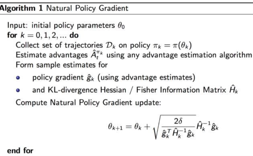
算法¶

训练 NPG 的完整算法如算法 1 所示：

在 XuanCe 中运行 NPG¶

在 XuanCe 中运行 NPG 之前，需要先准备一个 conda 环境，并按照 安装步骤安装 xuance。

运行内置示例¶

完成安装后，可以打开 Python 控制台，并使用以下命令直接运行 NPG：

import xuance
runner = xuance.get_runner(method='npg',
                           env='classic_control',  # 可选项：classic_control、box2d、atari。
                           env_id='CartPole-v1',  # 可选项：CartPole-v1、LunarLander-v2、ALE/Breakout-v5 等。
                           is_test=False)
runner.run()  # 也可以使用 runner.benchmark()

使用自定义配置运行¶

如需使用不同配置运行 NPG，可以新建一个 .yaml 文件，例如 my_config.yaml。然后使用以下代码运行 NPG：

import xuance as xp
runner = xp.get_runner(method='npg',
                       env='classic_control',  # 可选项：classic_control、box2d、atari。
                       env_id='CartPole-v1',  # 可选项：CartPole-v1、LunarLander-v2、ALE/Breakout-v5 等。
                       config_path="my_config.yaml",  # 请确保 my_config.yaml 文件的路径正确。
                       is_test=False)
runner.run()  # 也可以使用 runner.benchmark()

如需进一步了解配置方法，请参阅 配置教程。

在自定义环境中运行¶

如需在 XuanCe 尚未包含的自定义环境中运行 NPG，需要按照新环境教程 中的步骤定义新环境。然后，准备配置文件 npg_myenv.yaml。

完成上述操作后，可以使用以下代码在自定义环境中运行 NPG：

import argparse
from xuance.common import get_configs
from xuance.environment import REGISTRY_ENV
from xuance.environment import make_envs
from xuance.torch.agents import NPG_Agent

configs_dict = get_configs(file_dir="npg_myenv.yaml")
configs = argparse.Namespace(**configs_dict)
REGISTRY_ENV[configs.env_name] = MyNewEnv

envs = make_envs(configs)  # 创建并行环境。
Agent = NPG_Agent(config=configs, envs=envs)  # 创建一个来自 XuanCe 的 NPG 智能体。
Agent.train(configs.running_steps // configs.parallels)  # 对模型进行多个步骤的训练。
Agent.save_model("final_train_model.pth")  # 将模型保存到 model_dir。
Agent.finish()  # 结束训练。

参考文献¶

@article{kakade2001natural,
  title={A natural policy gradient},
  author={Kakade, Sham M},
  journal={Advances in neural information processing systems},
  volume={14},
  year={2001}
}