平均场 Q 学习 (MFQ)¶

论文链接: https://proceedings.mlr.press/v80/yang18d/yang18d.pdf

平均场多 Q 学习（MFQ）是一种改进的多智能体强化学习（MARL）算法，旨在解决传统多智能体 Q 学习的可扩展性和复杂性挑战。它引入了”平均场近似”来建模所有智能体的集体行为，而不是显式考虑每对智能体之间的交互，从而简化了大规模多智能体系统中的学习过程。

下表列出了 MFQ 算法的一些一般特性：

MFQ 的特性	值	描述
同策略	❌	评估策略与目标策略相同。
异策略	✅	评估策略与目标策略不同。
无模型	✅	不需要准备环境动力学模型。
基于模型	❌	需要环境模型来训练策略。
离散动作	✅	处理离散动作空间。
连续动作	❌	处理连续动作空间。

纳什 Q 学习¶

纳什均衡是博弈论的核心概念，指的是没有参与者可以通过单方面改变策略来提高自己收益的稳定状态。在随机博弈中，纳什均衡描述如下：

\[ v^j(s; \mathbf{\pi}_{*}) = v^j(s; \pi_{*}^j, \mathbf{\pi}_{*}^{-j}) \geq v^j(s; \pi^j, \mathbf{\pi}_{*}^{-j}) \]

这里，\(s\) 是状态，\(\pi_*\) 是所有智能体采用均衡策略（其中 \(\pi_*^{j}\) 是智能体 \(j\) 的均衡策略，\(\pi_*^{-j}\) 是除 \({j}\) 外所有智能体的均衡策略配置），\(v^{j}(s,\pi_*)\) 是智能体 \(j\) 的价值。这个公式可以理解为：没有智能体可以通过单方面改变策略来增加其在当前状态下的价值。

在纳什均衡中，给定纳什策略 \(\pi_*\)，纳什价值函数 \(\mathbf{v}^{nash}(s)\triangleq[v^{1}_{\pi_*}(s),\dots,v^{N}_{\pi_*}(s)]\)，纳什价值函数表示 Q 函数：

\[ \mathcal{H}^{\text{Nash}} \mathbf{Q}(s, \mathbf{a}) = \mathbb{E}_{s' \sim p} \left[ \mathbf{r}(s, \mathbf{a}) + \gamma \mathbf{v}^{\text{Nash}}(s') \right] \]

这里，\(\begin{cases} \mathbf{Q} \triangleq [Q^1, \dots, Q^N], \\ \mathbf{r}(s, \mathbf{a}) \triangleq [r^1(s, \mathbf{a}), \dots, r^N(s, \mathbf{a})]\end{cases}\)

平均场 MARL¶

联合动作空间的维度与智能体数量 \(N\) 成比例增长。为了解决这个问题，Q 函数通过仅利用成对局部交互进行分解：

\[ Q^{j}(s, \mathbf{a}) = \frac{1}{N^{j}} \sum_{k \in \mathcal{N}(j)} Q^{j}(s, a^{j}, a^{k}) \]

其中 \(\mathcal{N}(j)\) 是智能体 \(j\) 的邻居智能体的索引集，其大小 \(N(j)=|\mathcal{N}(j)|\) 由不同应用的设置决定。

平均场近似¶

计算 \(Q^{j}(s, \mathbf{a})\) 关于动作 \(a_k=\bar{a}^j\) 的二阶泰勒导数：

\[\begin{split} \begin{aligned} Q^j(s,\mathbf{a}) = \frac{1}{N^j} \sum_k Q^j(s, a^j, a^k) \\ & = \frac{1}{N^j} \sum_k \left[ Q^j(s, a^j, \bar{a}^j) + \nabla_{\bar{a}^j} Q^j(s, a^j, \bar{a}^j) \cdot \delta a^{j,k} + \frac{1}{2} \delta a^{j,k} \cdot \nabla_{ \tilde{a}^{j,k}}^2 Q^j(s, a^j, \tilde{a}^{j,k}) \cdot \delta a^{j,k} \right] \\ & = Q^j(s, a^j, \bar{a}^j) + \nabla_{\bar{a}^j} Q^j(s, a^j, \bar{a}^j) \cdot \left[ \frac{1}{N^j} \sum_k \delta a^{j,k} \right] + \frac{1}{2N^j} \sum_k \left[ \delta a^{j,k} \cdot \nabla_{\tilde{a}^{j,k}}^2 Q^j(s, a^j, \tilde{a}^{j,k}) \cdot \delta a^{j,k} \right] \\ & = Q^j(s, a^j, \bar{a}^j) + \frac{1}{2N^j} \sum_k R^j_{s,a^j}(a^k) \approx Q^j(s, a^j, \bar{a}^j) \end{aligned} \end{split}\]

其中，\(\sum_k R^j_{s,a^j}(a^k) \triangleq \sum_k \left[ \delta a^{j,k} \cdot \nabla_{\tilde{a}^{j,k}}^2 Q^j(s, a^j, \tilde{a}^{j,k}) \cdot \delta a^{j,k} \right] \) 表示泰勒多项式的余项，\(\tilde{a}^{j,k} = \bar{a}^{j} + \epsilon^{j,k} \delta a^{j,k}\)，\(\epsilon^{j,k} \in [0,1]\)。这里，使用 one-hot 编码表示 \(a^j\)：\(a^j \triangleq [a_1^j, \dots, a_N^j]\)，\(\bar{a}^j\) 是智能体的邻居 \(\mathcal{N}(j)\) 的平均动作。每个邻居的动作 \(a_k\) 表示为 \(\bar{a}^j\) 和小的波动 \(\delta a^{j,k}\) 的和：

\[ a^k = \bar{a}^j + \delta a^{j,k}, \quad \text{其中} \ \bar{a}^j = \frac{1}{N^j} \sum_k a^k \]

因此，许多智能体交互被有效地转换为两个智能体交互，\(Q^j(s,\mathbf{a})\approx Q^j(s, a^j, \bar{a}^j)\)。开发实用的平均场 Q 学习和平均场执行器-评判器算法。

Q 函数的迭代¶

MFQ 算法通过时序差分（TD）学习更新 Q 函数，其核心思想是”使用当前估计的未来 Q 值来修正当前的 Q 值”。此时，给定经验 \(e = (s, \{a^{k}\}, \{r^{j}\}, s')\)，平均场 Q 函数的更新函数为：

\[ Q_{t+1}^j(s, a^j, \bar{a}^j) = (1 - \alpha) Q_t^j(s, a^j, \bar{a}^j) + \alpha \left[ r^j + \gamma v^j_t(s') \right] \]

其中 \(\alpha\) 是学习率，\(\gamma\) 是折扣因子，平均场价值函数 \( v^j(s')\) 是：

\[ v_t^j(s') = \sum_{a^j} \pi^j_t(a^j | s', \bar{a}^j) \mathbb{E}_{\bar{a}^j(\mathbf{a}^{-j}) \sim \ \mathbf{\pi}^{-j}} \left[ Q_t^j(s', a^j,\bar{a}^j) \right] \]

为了区别于纳什价值函数 \(\mathbf{v}^{\text{Nash}}(s)\)，将上述公式表示为 \(\mathbf{v}^{\text{MF}}(s)\triangleq[v^1(s),\dots,v^N(s)]\)。定义平均场算子 \(\mathcal{H}^{\text{MF}}:\mathcal{H}^{\text{MF}}\mathbf{Q}(s, \mathbf{a}) = \mathbb{E}_{s' \sim p} \left[ \mathbf{r}(s, \mathbf{a}) + \gamma \mathbf{v}^{\text{MF}}(s') \right]\)。实际上，当 \(\mathcal{H}^{\text{MF}}\) 形成收缩映射时，即通过迭代应用平均场算子 \(\mathcal{H}^{\text{MF}}\) 来更新 \(\mathbf{Q}\)，平均场 Q 函数最终会在某些假设下收敛到纳什 Q 值。（具体假设和收敛证明可以在论文中找到。）

策略更新¶

为了平衡探索和利用，MFQ 通常采用玻尔兹曼（Softmax）策略来选择动作。为每个智能体 \(j\) 确定新的玻尔兹曼策略：

\[ \pi_t^j(a^j | s, \bar{a}^j) = \frac{\exp\left(-\beta Q_t^j(s, a^j, \bar{a}^j)\right)}{\sum_{a^{j'} \in \mathcal{A}^j} \exp\left(-\beta Q_t^j(s, a^{j'}, \bar{a}^j)\right)} \]

这里，\(\beta\) 是探索率。

这里，定义了一个迭代过程来计算 \(\bar{a}^j\)（智能体 \(j\) 的 \(N_j\) 个邻居来自由它们之前的平均动作 \({\bar{a}^k}_\_\) 参数化的策略 \(\pi^k_t\)）：

\[ \bar{a}^j = \frac{1}{N^j} \sum_k a^k, a^k \sim \pi_t^k(\cdot |s,{\bar{a}^k}_\_) \]

MFQ 借鉴了深度强化学习中 DQN 的稳定训练技术，并采用了经验回放和目标网络的思想。

通过与环境交互，执行联合动作 \(\mathbf{a} = [a^1, \dots, a^N]\)，并观察奖励 \(\mathbf{r} = [r^1, \dots, r^N]\) 和下一个状态 \(s'\)。将经验元组 \((s, \mathbf{a}, \mathbf{r}, s', \mathbf{\bar{a}})\) 存储在经验回放缓冲区 \(\mathcal{D}\) 中（其中 \(\mathbf{\bar{a}}\) = \([\bar{a}^1, \dots, \bar{a}^N]\) 是所有智能体的平均动作集）。

更新 Q 网络¶

采样经验：从经验回放缓冲区 \(\mathcal{D}\) 中采样小批次经验 \((s, \mathbf{a}, \mathbf{r}, s', \mathbf{\bar{a}})\)
继承平均动作：从目标网络 \(Q_{\phi^j_-}\) 中采样动作 \(a^j_-\)，并让目标网络继承当前的平均动作估计。

在 MFQ 中，智能体 \(j\) 通过最小化损失函数进行训练：

\[ \mathcal{L}(\phi^j) = \left( y^j - Q_{\phi^j}(s, a^j, \bar{a}^j) \right)^2 \]

其中 \(y^j = r^j + \gamma v_{\phi^j_-}^{\text{MF}}(s')\)，\(\phi^j_-\) 是目标网络的参数。

最后，不要忘记更新目标网络的参数：

\[ \phi^j_- \leftarrow \tau \phi^j + (1 - \tau) \phi_-^{j} \]

这里，\(\tau\) 是学习率。

MFQ 的优势：

该算法采用 Q 学习作为其框架，学习 Q 函数来指导动作选择，并使用时序差分误差更新 Q 值。
该算法采用平均场理论，使用”集体动作的平均值”来近似其他智能体对当前智能体的影响，从而解决多智能体场景中的状态空间爆炸问题。
借鉴 DQN 的稳定训练技术，如经验回放和目标网络。

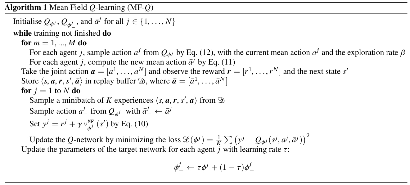
算法¶

MFQ 的完整训练算法如算法 1 所示：

_static/figures/pseucodes/pseucode-MFQ.png

在 XuanCe 中运行 MFQ¶

在 XuanCe 中运行 MFQ 之前，您需要准备 conda 环境并按照 安装步骤 安装 xuance。

运行内置演示¶

完成安装后，您可以打开 Python 控制台并使用以下命令直接运行 MFQ：

import xuance
runner = xuance.get_runner(method='mfq',
                           env='classic_control',  # 选择：claasi_control, box2d, atari.
                           env_id='CartPole-v1',  # 选择：CartPole-v1, LunarLander-v2, ALE/Breakout-v5 等。
                           is_test=False)
runner.run()  # 或 runner.benchmark()

要了解更多关于配置的信息，请访问 配置教程。

使用自定义环境运行¶

如果您想在 XuanCe 中未包含的自己的环境中运行 XuanCe 的 MFQ，您需要按照 新环境教程 中的步骤定义新环境。然后，准备配置文件 mfq_myenv.yaml。

之后，您可以使用以下代码在自己的环境中运行 MFQ：

import argparse
from xuance.common import get_configs
from xuance.environment import REGISTRY_ENV
from xuance.environment import make_envs
from xuance.torch.agents import MFQ_Agent

configs_dict = get_configs(file_dir="mfq_myenv.yaml")
configs = argparse.Namespace(**configs_dict)
REGISTRY_ENV[configs.env_name] = MyNewEnv

envs = make_envs(configs)  # 创建并行环境。
Agent = MFQ_Agent(config=configs, envs=envs)  # 从 XuanCe 创建 MFQ 智能体。
Agent.train(configs.running_steps // configs.parallels)  # 训练模型多个步骤。
Agent.save_model("final_train_model.pth")  # 将模型保存到 model_dir。
Agent.finish()  # 完成训练。

引用¶

@InProceedings{pmlr-v80-yang18d,
  title = 	 {Mean Field Multi-Agent Reinforcement Learning},
  author = 	 {Yang, Yaodong and Luo, Rui and Li, Minne and Zhou, Ming and Zhang, Weinan and Wang, Jun},
  booktitle = 	 {Proceedings of the 35th International Conference on Machine Learning},
  pages = 	 {5571-5580},
  year = 	 {2018},
  editor = 	 {Dy, Jennifer and Krause, Andreas.},
  volume = 	 {80},
  series = 	 {International Conference on Machine Learning},
  address = 	 {Stockholmsmässan, Stockholm Sweden},
  month = 	 {10--15 July},
  publisher =    {PMLR},
  pdf = 	 {https://proceedings.mlr.press/v80/yang18d/yang18d.pdf},
  url = 	 {https://proceedings.mlr.press/v80/yang18d.html},
  abstract = 	 {Existing multi-agent reinforcement learning methods are limited typically to a small number of agents. When the agent number increases largely, the learning becomes intractable due to the curse of the dimensionality and the exponential growth of agent interactions. In this paper, we present Mean Field Reinforcement Learning where the interactions within the population of agents are approximated by those between a single agent and the average effect from the overall population or neighboring agents; the interplay between the two entities is mutually reinforced: the learning of the individual agent's optimal policy depends on the dynamics of the population, while the dynamics of the population change according to the collective patterns of the individual policies. We develop practical mean field Q-learning and mean field Actor-Critic algorithms and analyze the convergence of the solution to Nash equilibrium. Experiments on Gaussian squeeze, Ising model, and battle games justify the learning effectiveness of our mean field approaches. In addition, we report the first result to solve the Ising model via model-free reinforcement learning methods.}
}